TDSM 6.1
6-1. Provide answers to the questions associated with the following data sets, available at http://www.data-manual.com/data:
a. Analyze the movie data set. What is the range of movie gross in the U.S.? Which type of movies are most likely to succeed in the market? Comedy? PG-13? Drama?
The range of U.S. movie gross in this data set is 0 to 760167650, presumably in U.S. dollars. However, the records of 0 are likely incomplete or perhaps movies that were never released in the United States. So, after removing rows that include 0 or “Unknown”, we’ll say the range is 401 to 760167650 (further munging may yield an even higher minimum).
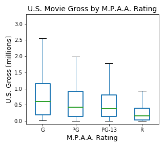
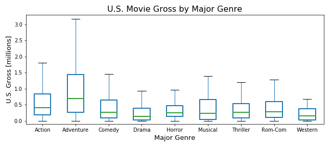
Let’s consider "success in the market" to be a relative comparison of U.S. Movie Gross between movies and the "type" to be based on the M.P.A.A. Rating and Major Genre. At a glance, we can see that the top 3 grossing movies as well as most of the top 100 are rated PG-13. We also see that the Adventure genre appears most frequently in the top 100. But if we are talking about most likely to succeed in relation to all movies, then we want to know more about the distribution of gross over all movies for each type, rather than just the outliers. We can get a clear view of this by creating box plots that don't display outliers.
We can see that Adventure movies tend to gross more than other genres, which is consistent with the top 100. However, G rated movies gross more than other ratings, which is different than in the top 100. Further analysis, such as applying inflation to gross based on release date or factoring in production budget may yield different results, but based on these results we can say that Adventure movies and G rated movies are most likely to succeed in the market.
b. Analyze the Manhattan rolling sales data set. Where in Manhattan is the most/least expensive real estate located? What is the relationship between sales price and gross square feet?
Looking over this data set, we can see a lot of incomplete records, duplicate records, and strange data, particularly in the “SALE PRICE” column. Some properties sell for millions of dollars, while others in the same neighborhood with similar attributes sell for $100, $10, or even $0. If we navigate the website http://www1.nyc.gov/site/finance/taxes/property-rolling-sales-data.page that released the data set, we come across a glossary that explains each column, as well as somewhat of an explanation for this phenomenon in sales price.
From the glossary, “A $0 sale indicates that there was a transfer of ownership without a cash consideration. There can be a number of reasons for a $0 sale including transfers of ownership from parents to children.” [1]
This explains $0 sales, but may also explain situations where sales are close to $0 or seem low relative to their other attributes. Since it is not practical to perform imputation such as interpolating more “correct” values, nor is it necessarily relevant to answer the question, we can perform our analysis without any extraneous munging.
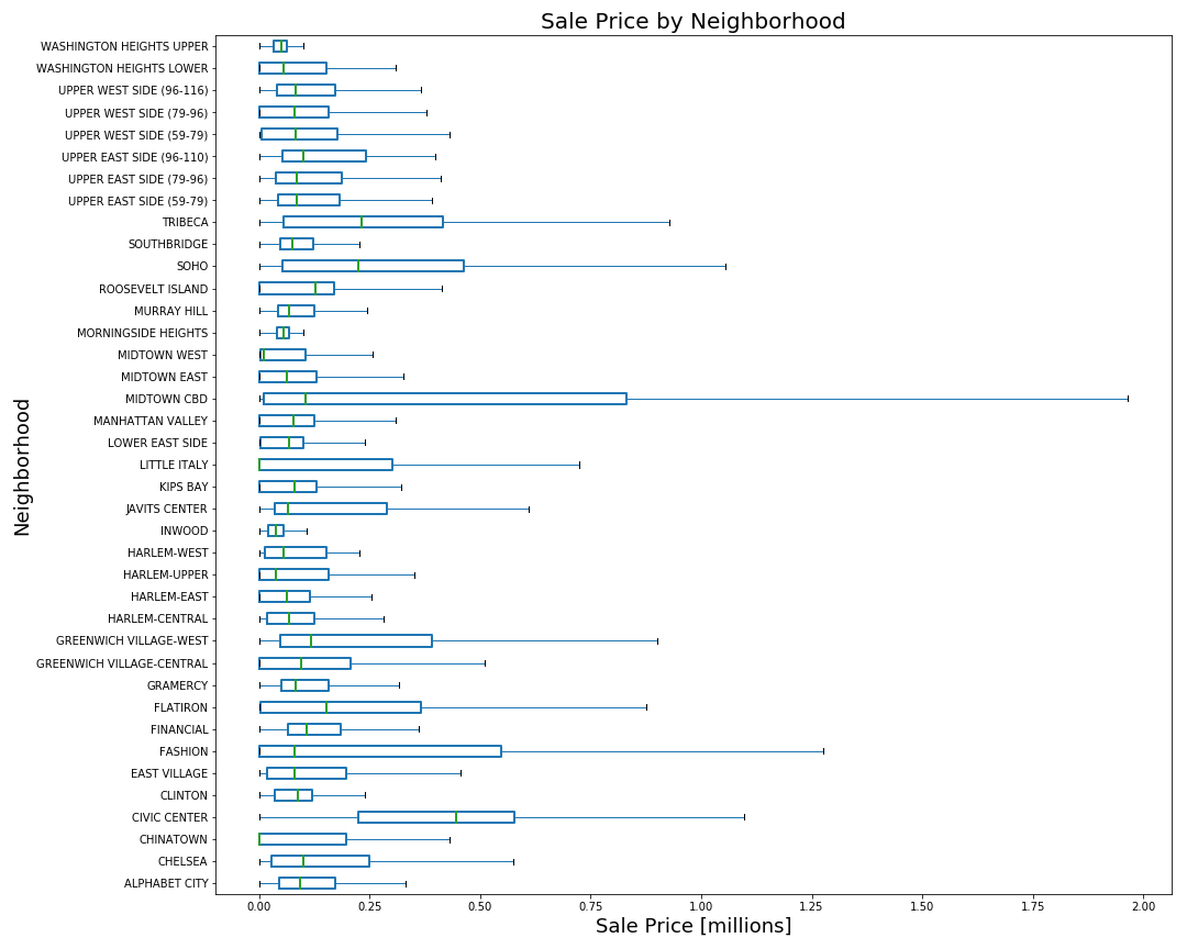
Since we have a large numbers of variables (neighborhoods) with long names, we can plot their sales price distribution as a horizontal box plot.
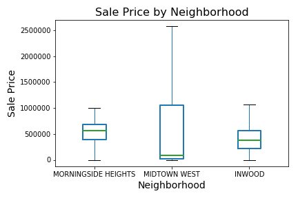
It is clear from this plot that Midtown CBD has the most expensive real estate, but it is hard to determine where the lowest real estate is. We can take the 3 lowest appearing neighborhoods and plot them similarly to get a closer look.
Here we get a more precise view and can see that while Midtown West has the highest maximum of the three, the sales are more greatly distributed in a lower range than the other two neighborhoods. With this information, we can say that the most expensive real estate is located in Midtown CBD and the least expensive in Midtown West.
To determine the relationship between sales price and gross square feet, we can calculate the Pearson correlation coefficient between the two columns in the data set. This yields a value of 0.594686970478, which indicates a positive linear relationship between sales price and gross square feet.
c. Analyze the 2012 Olympic dataset. What can you say about the relationship between a country's population and the number of medals it wins? What can you say about the relationship between the ratio of female and male counts and the GDP of that country?
d. Analyze the GDP per capita dataset. How do countries from Europe, Asia, and Africa compare in the rates of growth in GDP? When have countries faces substantial changes in GDP, and what historical events were likely most responsible for it?


